snazzieR
Chic and Sleek Functions for Beautiful Statisticians
Because your linear models deserve better than console output. A sleek color palette and kable styling to make your regression results look sharper than they are.
Installation
Get started with snazzieR
PLS Regression
SVD & NIPALS algorithms
Plot Theme
Themes and color palettes
Examples
Usage examples and tutorials
About snazzieR
snazzieR is an R package designed to make your statistical analysis outputs beautiful and publication-ready. It includes support for Partial Least Squares (PLS) regression via both the SVD and NIPALS algorithms, along with a unified interface for model fitting and fabulous LaTeX and console output formatting.
The package provides a comprehensive suite of functions for PLS regression analysis, including both SVD and NIPALS algorithms, cross-validation capabilities, and beautiful output formatting for both LaTeX and console display. Whether you're working on academic research or industry applications, snazzieR helps you create publication-ready results with minimal effort.
Installation
# Install from CRAN
install.packages("snazzieR")

# Load the package
library(snazzieR)
Partial Least Squares (PLS) Regression
Overview
PLS regression is a dimension reduction technique that projects predictors to a lower-dimensional space that maximally explains covariance with the response variable(s). It's especially useful when:
- Predictors are highly collinear
- The number of predictors exceeds the number of observations
- You need interpretable latent variables
pls.regression
The main user-facing function for computing PLS models. Provides a unified interface for both SVD and NIPALS algorithms.
Usage:
pls.regression(x, y, n.components = NULL, calc.method = c("SVD", "NIPALS"))Arguments:
- x: A numeric matrix or data frame of predictor variables (X), with dimensions n × p
- y: A numeric matrix or data frame of response variables (Y), with dimensions n × q
- n.components: Integer specifying the number of latent components (H) to extract. If NULL, defaults to the rank of x
- calc.method: Character string indicating the algorithm to use. Must be either "SVD" (default) or "NIPALS"
Returns:
- model.type: Character string ("PLS Regression")
- T, U: Score matrices for X and Y
- W, C: Weight matrices for X and Y
- P_loadings, Q_loadings: Loading matrices
- B_vector: Component-wise regression weights
- coefficients: Final regression coefficient matrix (rescaled)
- intercept: Intercept vector (typically zero due to centering)
- X_explained, Y_explained: Variance explained by each component
- X_cum_explained, Y_cum_explained: Cumulative variance explained
SVD Method
A direct method using the singular value decomposition of the cross-covariance matrix (X^T Y).
- • Computes all components at once
- • More efficient for large datasets
- • Numerically stable
- • Default method
NIPALS Method
An iterative method that alternately estimates predictor and response scores until convergence.
- • Computes components one at a time
- • Handles missing data well
- • Memory efficient
- • Original PLS algorithm
pls.summary
Formats and displays Partial Least Squares (PLS) model output as either LaTeX tables (for PDF rendering) or console-friendly output. Provides comprehensive model diagnostics and component analysis.
Usage:
pls.summary(x, include.scores = TRUE, latex = TRUE)Example:
# Prepare iris data for PLS regression
x.iris <- iris[, c("Sepal.Length", "Sepal.Width")]
y.iris <- iris[, c("Petal.Length", "Petal.Width")]
x.mat.iris <- as.matrix(x.iris)
y.mat.iris <- as.matrix(y.iris)

# Fit PLS model using NIPALS algorithm
NIPALS.pls.iris <- pls.regression(
  x.mat.iris,
  y.mat.iris,
  n.components = 3,
  calc.method = "NIPALS"
)

# Generate PLS summary (exclude scores for cleaner output)
pls.summary(NIPALS.pls.iris, include.scores = FALSE)
Cross Validation
The package includes custom K-fold cross-validation utilities for model evaluation and selection.
Functions:
- create_kfold_splits: Creates K-fold cross-validation splits
- kfold_cross_validation: Performs K-fold cross-validation with customizable metrics
Statistical Analysis Functions
ANOVA.summary.table
Generate a summary table for ANOVA results, including degrees of freedom, sum of squares, mean squares, F-values, and p-values.
Usage:
ANOVA.summary.table(model, caption, latex = TRUE)Example:
# Fit a linear model
model <- lm(mpg ~ wt + hp, data = mtcars)

# Generate a plain-text ANOVA summary table
ANOVA.summary.table(model, caption = "ANOVA Summary", latex = FALSE)
model.summary.table
Generate a summary table for a linear model, including estimated coefficients, standard errors, p-values with significance codes, and model statistics. Perfect for publication-ready output.
Usage:
model.summary.table(model, caption = NULL, latex = TRUE)Example:
# Fit a linear model using iris data
iris.lm <- lm(Petal.Length ~ Sepal.Length + Sepal.Width, data = iris)

# Generate LaTeX-formatted summary table
model.summary.table(iris.lm, caption = "Linear Regression Model Summary")

# Print to console
model.summary.table(iris.lm, caption = "Linear Model Summary", latex = FALSE)
model.equation
Generate a model equation from a linear model object with options for LaTeX formatting. Creates publication-ready mathematical equations.
Usage:
model.equation(model, latex = TRUE)Example:
# Fit a linear model using iris data
iris.lm <- lm(Petal.Length ~ Sepal.Length + Sepal.Width, data = iris)

# Generate LaTeX equation
model.equation(iris.lm)

# Print equation to console
model.equation(iris.lm, latex = FALSE)
eigen.summary
Computes summary statistics for eigenvalues from a correlation or covariance matrix, providing descriptive statistics and percentage of variance explained. Essential for principal component analysis and dimension reduction techniques.
Usage:
eigen.summary(correlation_matrix)Example:
# Prepare iris data and standardize
iris.data <- iris[, 1:4]
scaled.data <- as.data.frame(
  lapply(iris.data, function(x) {
    (x - mean(x)) / sd(x)
  })
)
correlation.matrix <- cor(scaled.data)

# Generate eigenvalue analysis
eigen.summary(correlation.matrix)
Plot Theme & Styling
Color Palette
snazzieR includes a collection of 35 named hex colors grouped by hue and tone. Each color is available as an exported object (e.g., Red, Dark.Red). The color.ref() function produces a comprehensive color palette plot showing all colors with their hex codes.
Red Family
Orange Family
Yellow Family
Green Family
Blue Family
Purple Family
Grey Family
Color Reference Plot
Plot produced by color.ref() showing all 35 colors:
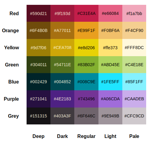
Color Reference Function
color.ref()Displays a comprehensive color palette plot showing all 35 colors with their hex codes, organized in a grid format.
snazzieR Theme
snazzieR.theme
A custom ggplot2 theme for publication-ready plots with a clean, polished look focused on readability and aesthetics.
Usage:
snazzieR.theme()Example:
# Load required libraries
library(ggplot2)
library(dplyr)
library(gridExtra)
library(grid)
library(snazzieR)
# Create individual plots with snazzieR theme and colors
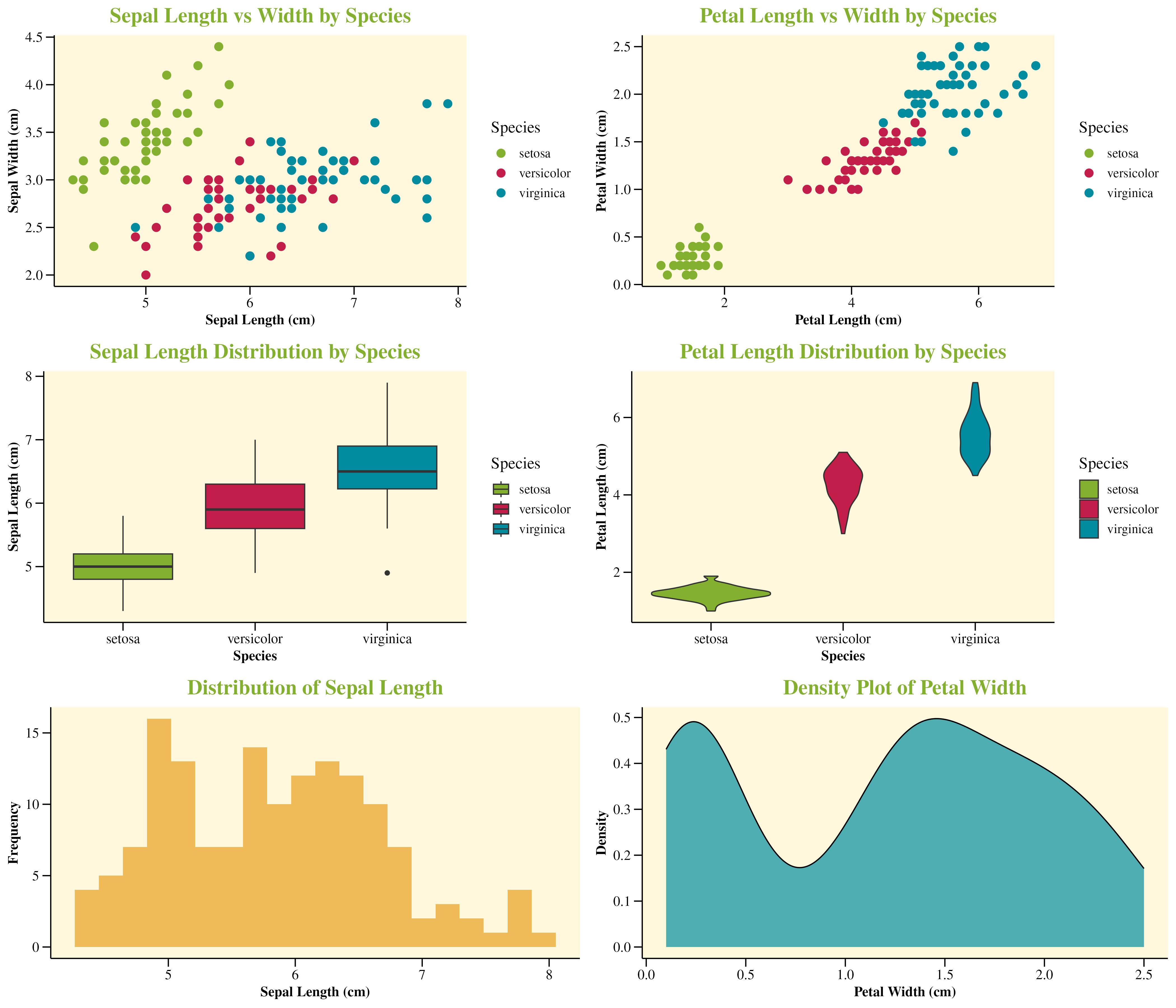
p1 <- ggplot(iris, aes(x = Sepal.Length, y = Sepal.Width, color = Species)) +
geom_point(size = 3) +
scale_color_manual(values = c(
"setosa" = snazzieR::Green,
"versicolor" = snazzieR::Red,
"virginica" = snazzieR::Blue
)) +
labs(
title = "Sepal Length vs Width by Species",
x = "Sepal Length (cm)",
y = "Sepal Width (cm)"
) +
snazzieR::snazzieR.theme()
p2 <- ggplot(iris, aes(x = Petal.Length, y = Petal.Width, color = Species)) +
geom_point(size = 3) +
scale_color_manual(values = c(
"setosa" = snazzieR::Green,
"versicolor" = snazzieR::Red,
"virginica" = snazzieR::Blue
)) +
labs(
title = "Petal Length vs Width by Species",
x = "Petal Length (cm)",
y = "Petal Width (cm)"
) +
snazzieR::snazzieR.theme()
p3 <- ggplot(iris, aes(x = Species, y = Sepal.Length, fill = Species)) +
geom_boxplot() +
scale_fill_manual(values = c(
"setosa" = snazzieR::Green,
"versicolor" = snazzieR::Red,
"virginica" = snazzieR::Blue
)) +
labs(
title = "Sepal Length Distribution by Species",
x = "Species",
y = "Sepal Length (cm)"
) +
snazzieR::snazzieR.theme()
p4 <- ggplot(iris, aes(x = Species, y = Petal.Length, fill = Species)) +
geom_violin() +
scale_fill_manual(values = c(
"setosa" = snazzieR::Green,
"versicolor" = snazzieR::Red,
"virginica" = snazzieR::Blue
)) +
labs(
title = "Petal Length Distribution by Species",
x = "Species",
y = "Petal Length (cm)"
) +
snazzieR::snazzieR.theme()
p5 <- ggplot(iris, aes(x = Sepal.Length)) +
geom_histogram(bins = 20, fill = snazzieR::Orange, alpha = 0.7) +
labs(
title = "Distribution of Sepal Length",
x = "Sepal Length (cm)",
y = "Frequency"
) +
snazzieR::snazzieR.theme()
p6 <- ggplot(iris, aes(x = Petal.Width)) +
geom_density(fill = snazzieR::Blue, alpha = 0.7) +
labs(
title = "Density Plot of Petal Width",
x = "Petal Width (cm)",
y = "Density"
) +
snazzieR::snazzieR.theme()
# Arrange plots in a grid
grid.arrange(p1, p2, p3, p4, p5, p6, ncol = 2, nrow = 3)Iris Visualization Examples
Examples of snazzieR visualizations using the iris dataset, showcasing the color palette and theme in action.
Examples & Tutorials
Iris Data Analysis
Source: Fisher, R. (1936). Iris [Dataset]. UCI Machine Learning Repository.https://doi.org/10.24432/C56C76
# Load required libraries
library(ggplot2)
library(dplyr)
library(gridExtra)
library(grid)
library(snazzieR)
library(kableExtra)

# Prepare iris data
data(iris)
x.iris <- iris[, c("Sepal.Length", "Sepal.Width")]
y.iris <- iris[, c("Petal.Length", "Petal.Width")]
x.mat.iris <- as.matrix(x.iris)
y.mat.iris <- as.matrix(y.iris)
Iris Dataset Preview
Dataset Structure
The iris dataset contains measurements for 150 iris flowers from three different species. Each flower has four measurements: sepal length, sepal width, petal length, and petal width.
# Display first 6 observations with dots
iris.table <- head(cbind(x.iris, y.iris))
dots.row <- as.data.frame(matrix("\vdots", nrow = 1, ncol = ncol(iris.table)))
colnames(dots.row) <- colnames(iris.table)
iris.table.with.dots <- rbind(iris.table, dots.row)
colnames(iris.table.with.dots) <- gsub("\.", " ", colnames(iris.table.with.dots))

# Create formatted table
kable(
  iris.table.with.dots,
  caption = "Iris Dataset (First 6 Observations): Predictors and Responses",
  booktabs = TRUE,
  linesep = "",
  format = "latex",
  align = "c",
  escape = FALSE
) %>%
  kable_styling(
    latex_options = c("HOLD_position", "striped"),
    full_width = FALSE,
    position = "center",
    font_size = 12
  )
Output
Linear Regression Analysis
Code Example
# Fit linear regression model
iris.lm <- lm(Petal.Length ~ Sepal.Length + Sepal.Width, data = iris)

# Model summary table
snazzieR::model.summary.table(iris.lm, caption = "Linear Regression Model Summary")
Output
Model Equation
Code Example
# Generate model equation
snazzieR::model.equation(iris.lm)
Output
ANOVA Analysis
Code Example
# Generate ANOVA summary table
snazzieR::ANOVA.summary.table(iris.lm, caption = "ANOVA Results")
Output
Eigenvalue Analysis
Code Example
# Prepare iris data and standardize
iris.data <- iris[, 1:4]
scaled.data <- as.data.frame(
  lapply(iris.data, function(x) {
    (x - mean(x)) / sd(x)
  })
)
correlation.matrix <- cor(scaled.data)

# Eigenvalue analysis
snazzieR::eigen.summary(correlation.matrix)
Output
PLS Regression (NIPALS)
Code Example
# Fit PLS model using NIPALS algorithm
NIPALS.pls.iris <- snazzieR::pls.regression(
  x.mat.iris,
  y.mat.iris,
  n.components = 3,
  calc.method = "NIPALS"
)

# Generate PLS summary
snazzieR::pls.summary(NIPALS.pls.iris, include.scores = FALSE)
Output
Technical Details
SVD Algorithm
The SVD method computes latent variables using the singular value decomposition of the cross-covariance matrix (X^T Y).
- Z-score standardization of X and Y
- Compute cross-covariance matrix R = E^T F
- Perform SVD: R = U D V^T
- Extract first singular vectors: w = U[,1], q = V[,1]
- Compute scores: t = E w (normalized), u = F q
- Compute loadings and deflate residuals
NIPALS Algorithm
The NIPALS method iteratively estimates predictor and response scores until convergence.
- Initialize random response score vector u
- Update X weight vector: w = E^T u (normalized)
- Compute X score: t = E w (normalized)
- Update Y loading: q = F^T t (normalized)
- Update response score: u = F q
- Repeat until t converges
Package Structure
Core Functions:
- pls.regression: Main PLS interface
- SVD.pls: SVD-based PLS implementation
- NIPALS.pls: NIPALS algorithm implementation
- pls.summary: Output formatting
- format.pls: LaTeX/console formatting
References & Links
Academic References
- • Abdi, H., & Williams, L. J. (2013). Partial least squares methods: Partial least squares correlation and partial least square regression. Methods in Molecular Biology, 930, 549–579.
- • de Jong, S. (1993). SIMPLS: An alternative approach to partial least squares regression. Chemometrics and Intelligent Laboratory Systems, 18(3), 251–263.
- • Fisher, R. A. (1936). The use of multiple measurements in taxonomic problems. Annals of Eugenics, 7(2), 179–188.
- • Wold, H., & Lyttkens, E. (1969). Nonlinear iterative partial least squares (NIPALS) estimation procedures. Bulletin of the International Statistical Institute, 43, 29–51.
Package Information
- • Maintainer: Aidan J. Wagner
- • License: MIT
- • R Version: ≥ 3.5
- • Version: 0.1.2
- • Dependencies: ggplot2, knitr, kableExtra, dplyr, stats